Use the proper formula in the cell I2 to display the number of the day of the week (Sunday=1,Monday=2,...), which appears in the cell A2.
Use the proper formula in the cell I2 to produce the date which appears in the cell A2 with an addition of 5 more working days.
Make sure the formula will consider only Sundays as non-working days.
Display the watch window and add the cell H2 in the watch list.
Use the Goal seek, to calculate the amount of the monthly payments, so that the period of the loan becomes 10 years.
Make sure that in the cell area A1:A10 of the Total Worksheet, the sums of the cells, of the respected cell areas of the sheets FF1,FF2,FF3,FF4 are displayed. Use Excel's Consolidate Tool.
Display in the proper cell area of the sheet Average, the average grades of the courses of the year. The grades per trimester are displayed in their respected sheets. Use Excel's Consolidate Tool (Include the 1st row in the reference areas).
In the cells B1:B6 set the values of the cell range A1:A6.
If their values cannot be represented by a number then set the value in the corresponding cell of the B column to 0.
You can use the conditional functions IF, ISERROR, IFERROR and the VALUE function.
Then calculate the sum of the cell range B1:B6 in the cell B8.
In the cells B2:B4 insert the appropriate function to return TRUE if the respective cell of the A column is a formula.
In the cells B2:B4 insert the appropriate function to return TRUE if the respective cell of the A column is text.
In the cells B2:B4 insert the appropriate function to return TRUE if the respective cell of the A column is blank.
In the cells B2:B4 insert the appropriate function to return TRUE if the respective cell of the A column has an error besides the #N/A error.
In the cells B2:B4 insert the appropriate function to return TRUE if the respective cell of the A column is an even number.
In the cells B2:B4 insert the appropriate function to return TRUE if the respective cell of the A column is a logical variable.
In the cells B2:B4 insert the appropriate function to return TRUE if the respective cell of the A column has a #N/A error.
In the cells B2:B4 insert the appropriate function to return TRUE if the respective cell of the A column is NOT text.
In the cells B2:B4 insert the appropriate function to return TRUE if the respective cell of the A column is number.
In the cells B2:B4 insert the appropriate function to return TRUE if the respective cell of the A column is an odd number.
Correct the error of the formula in cell D19 of the 2ndhour2 worksheet.
Display the sales of the Della company in the cell Â8 of the vlookup worksheet, with the use of the function vlookup. You will find the sales of the company in the SALES worksheet. Then reproduce the function up to the cell B12.
Display the representative of the Della company in the cell B8 of the hlookup workbook using the hlookup function. Representatives of companies are displayed in the SALES worksheet. Then reproduce the function up to the cell G8.
Use the Lookup function to display in the cell C20 the value of the Column C that corresponds to the letter of the Column A, according to the letter displayed in the A20 cell. The table range is A1:C18.
Format the cell range B1:B10 so that numbers are displayed with 4 decimal places and a thousand separator. Then insert the appropriate function in this cell range to display the difference in days between the date in column A and the current date and time.
Insert the appropriate function in the cell A1, to return the current date and time. Insert the appropriate function in the cell A2, to return the current date and time increased by 4 days (+ 4 days). Insert the appropriate function in the cell A3, to return the current date and time increased by 365 days (+ 365 days).
Insert an appropriate function in the cell E2 to return the date for the values of the cell range A2:C2. Reproduce the function in the cell range E3:E11.
Use the function date(), to insert the date 9 July 1968 in the cell C5.
There is a message for an error in the cell G6. The formula doesn’t contain any errors. Without changing the cell G6, find out which is the cell to cause the error and insert the appropriate formula or function in it.
Use the sumif function in the cell E15 to calculate the total points received by Gladbach .
The cell range G3:H8 displays teams and countries of origin. Insert a function in the cell D2 to return the country name for the specific team. Then, reproduce the function in the cell range D3:D21. Use the VLOOKUP function
Create two scenarios using the following data. The changing cells will be D7:D9. The first one, named Optimistic, will display:
value 1323 in the cell D7
value 543 in the cell D8
value 987 in the cell D9.
The second, named Pessimistic, will display:
value 989 in the cell D7
value 243 in the cell D8
value 890 in the cell D9.
Run mymacro in the cell B4.
Record a new macro using the name newmacro to apply Bold and Italics.
Find the circular reference error and correct it.
Use the proper excel function to make sure that the formula used in the cell B2 of the 2016 worksheet, is displayed in the cell B42.
In the cell H4 calculate the count of the orders, with amount greater than 40 that were placed after February 1st 2004.
Use the IFERROR formula to make sure that the cells C10:K10 show the number 0, when the sum of the sales of all the companies is 0 in one month, as for example in August.
In the cell H4 calculate the sum of all orders with amount greater than 40, which were placed after 2/1/2004.
In the worksheet there is information about a loan. Use the Goal Seek to calculate, in how many months the loan would be repaid if the required amount of monthly installments were 900 dollars.
Use the proper formula to match the position of the table where the products of the cells E7:E8 are found, and show the respected values in the cells F7:F8.
Use the proper formula in the cell F16 to calculate the sum of the values in the area with position: 1 column left and 11 rows above from the cell F16.
The area should be 5 rows high and 2 columns wide.
Use the proper function in cell E1 to calculate the value, of the cell in the second row and third column, of the cell range A1:D6.
Calculate all formulas in the sales sheet.
Calculate all formulas in the Workbook.
In the current sheet there is an error. Use error tracing to find its actual source.
Activate the error checking rule for formulas referring to empty cells.
In the active Sheet remove all tracing arrows.
Insert in the sheet Sheet2 a button form control item. It will execute the macro italic. Its caption should be Italic letters
Use the proper formula in the cell I2, to calculate the sum of the Total of Sales, from the eastern district, with less than 55 units sold.
Use the proper formula in the cell I2, to calculate the average of the Total of Sales, from the western district, with greater than 100 units sold.
Use the proper formula in the cell I2, to calculate the count of the Total of Sales, from the eastern district, with less than 80 units sold.
In the cell range G5:G10 use the proper formula, to calculate the number of periods (in months) for each one of the investments.
Insert your birthday date in the cell A1. Insert a function in the cell A2 that always displays the current date. Insert a function in the cell A3 that displays the number of the days you have lived. Format the cell A3 in Number category with a thousand separator and without decimals.
In the cell range B2:D21, insert the appropriate functions so that column B displays the day of the date appearing in column A, column C displays the month of the date appearing in column A, column D to displays the year of the date appearing in column A.
Insert the appropriate function in the cell A1 to sum up values greater than or equal to 5000 in the cell range A2:A100. Insert the appropriate function in the cell B1 to sum up the cells, the corresponding cells of which in column A display a value greater than or equal to 5000, in the cell range B2:B100.
Insert the appropriate functions in the cell range G5:G10 that return the monthly payments for a loan based on regular payments and stable interest rate. Necessary data are provided in the cell range B5:F10.
Insert the appropriate function in the cell E3 that returns the value TRUE if the content of cell A3 is greater than 10 and the content of cell B3 is greater than 10 and the content of cell C3 is greater than 10 and the content of cell D3 is TRUE. Otherwise the function should return the value FALSE.
Reproduce that function up to the cell E50. Finally, insert a function in the cell E1 that returns the value TRUE if the value TRUE is displayed at least once in the cell range E3:E50. (use only the AND and OR functions)
On the SALES worksheet trace the precedents of the cell J20. Also, trace the dependents of the cell F9.
Create two Scenarios with the following data:
1) Name: Min, changing cells: C5:C8, values: 5, 6, 10, 8 2) Name: Max, changing cells: C5:C8, values: 11, 12, 15, 10.
Display the scenario Max.
Create a scenario summary using the default values.
Navigate to the cell A13 and use the appropriate function to Count how many products are charged with a final price greater than 250€
Navigate to the cells C2:C14 and create a function that returns the respective Name of singer appearing in the cell range A18:B20. Use the VLOOKUP function
Use the appropriate function in the cell E11, to return the day of the date displayed in the cell E4.
Navigate to the SALES worksheet and insert a function in the cell E9 which derives data from the cell range C5:C24, in order to calculate the sum of sales achieved by the salesman Lambropoulos.
Apply a fill color of your choice on the cells depended by the cell D10.
Apply fill color of your choice on all the precedents of cell D27.
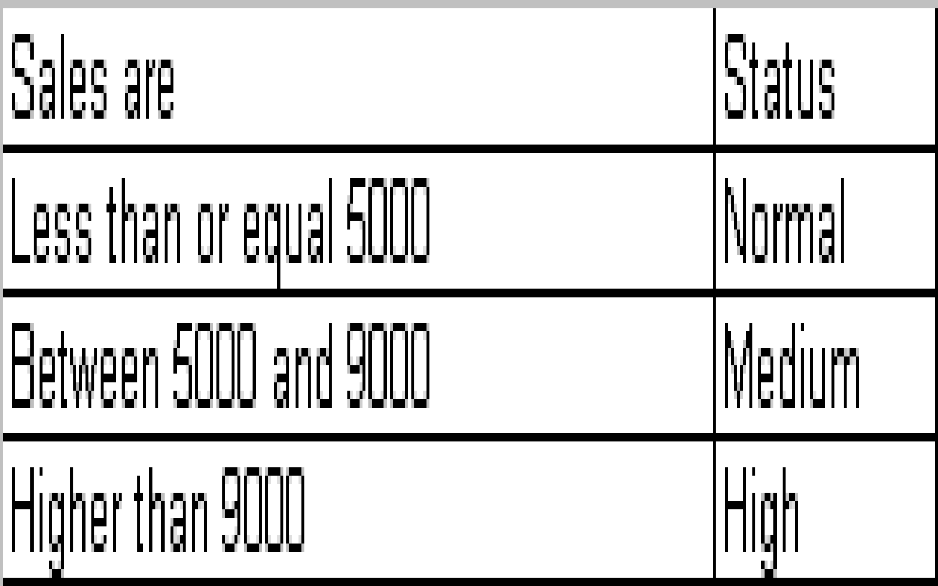
Enter the appropriate nested functions in the cell range D5:D16 to return the Expenses status as follows (do not use the IFS function):
Enter a function in the cell A1 to display the current date.
On the Sheet1 worksheet delete the scenario called Scenario1.
Add a keyboard shortcut for the macro mymacro using the Ctrl+b combination.
At the cell area B8:G8 of Sheet3 show the average grade of the lessons with grades greater than or equal to 5.
In the cell O18 using the proper combination of INDEX and MATCH functions lookup the income for the specific date shown in the cell O17 from the cell range B2:M32. Ensure that if we change the value in the cell O17 the value in the cell O18 will change respectively.
Complete the cells B3:B15 using the proper excel logical function.