We have reached the end of our quest for the best lookup function, where we will talk about the combination of INDEX and MATCH. In the current lesson, we will use INDEX with dual MATCH functions, to achieve a matrix lookup functionality. But you can easily skip one of the two MATCH functions, and replace it with a static value if you are not interested in a matrix lookup.
Practice File:
Transcript
The knowledge of the simple syntax of the functions mentioned, is considered a prerequisite.
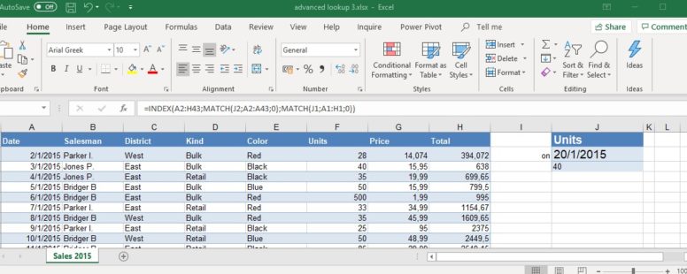
We are trying to find the number of units sold on January 20th of 2015.
In J3 we type the name of the function, and the cell area of our data which is, A2:H43.
For the row number, we will use our first match function.
We type match and set J2 as the lookup value, and the data of the first column as the lookup array, (A2:A43). We are looking for the exact match so we type “0”.
Next, for the column number, we use our second match function, with j1 as the lookup value and, A1:H1 as the lookup array.
We use 0 again, since we are looking for an exact match. We close the parenthesis and press enter.
The result, as expected, is 40. Kind of easy, isn’t it?
The limitation of all the other formulas for lookup is, that there is no easy way to do a right to left search.
Fortunately, this combination doesn’t suffer from the same disability.
Right to left search can be done as easily as left to right.
Suppose we want to find the date when we sold 500 units.
We use the same syntax as before, in cell J16. First the index function with our data array, and then the two match functions, for row and column number respectively.
For the first, the lookup value is found on L15, which are the 500 units, and lookup area the cells F2:F43. We are looking for an exact match, so the last attribute is set to 0.
For the column number, we type the match function again, with first attribute, the cell J15, and lookup array the A1:H1 cell range. Once more, we search for an exact match.
We close the parenthesis, and we have the required result.
Until Microsoft creates a built-in function, that matches or surpasses the versatility of index and match combination, I believe they are the best choice for any lookup scenario.
This concludes the chapter for lookup functionality in Excel, and I hope It was helpful to you. Stick around, for equally interesting stuff.