There is no way to create a powerful and versatile lookup formula without using at least once the MATCH function.
Practice File:
Transcript
Let us see now how exactly it works.
The match function looks up information from an array of data, just like the choose function we saw in a previous lesson.
The difference is that the match function returns the position of the lookup value in the array of data.
The match function also allows us to choose if it will return an exact match of the requested value, or the closest match (above or below) the requested value.
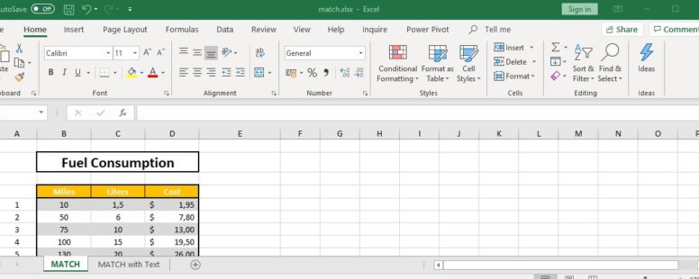
Let us see how it works. We need to find the position (row number) of the table where the cost is 13 dollars and show it in cell D15;
So in cell 15 we use the match function. For the first attribute we type the value 13 and as a lookup array we provide the cell range of the cost which is D5:D12.
Since we need the exact match of this cost we then select 0 as the final attribute.
The two other options we have is 1, which is the default and minus 1.
The result after we press enter is 3, which in such a small pool of data can easily see ourselves.
If instead of 13 dollars we searched for 15 the function would produce an error since it is looking for an exact match.
In this case we can change the final attribute to either 1 or minus 1.
If we change it to 1 then the function returns the closest match below or equal to the lookup value. For this to work the array must be sorted in ascending order.
If we set the attribute to “minus 1” then the function will return the closest match above or equal to the lookup value. The array in this case should be sorted in descending order.
In the first case the result remains 3 and it represents the position of the value 13 which is the closest match below 15.
In the second case the result is 5 and it represents the closest match above 15 which is 19.5.
Let’s see how good match works when searching for a text.
Suppose we have a list of our colleagues and their birthdays. We want to find the birthday of a friend whose name begins with the letters Yv and has a double n somewhere inside it, but we don’t remember it exactly.
Match can help us. In Cell E10 we type the function followed by the text we remember (Yv) followed by the asterisk character the double n and another asterisk character. Then we select the array of first names which is the cell range B2:B37 and for the last attribute we type 0 since we want the exact match.
The result is 11 and in the eleventh position we find Yvonne. Her birthday is on May 4 and she is a few weeks due on her present.
Match by itself is a function that a lot of us might think we will never actually use. But in combination with other functions it is a tool we simply cannot ignore, as we will see on the following lessons.