Excel provides us with 2 functions for calculating accrued interest. ACCRINT, ACCRINTM.
But what exactly is accrued interest?
Practice File:
Transcript
Accrued interest is the interest that has been earned, but not yet been paid by the bond issuer, since the last coupon payment. Because the security hasn’t expired or the next payment is not yet due, the owner hasn’t officially received the money. If he or she sells the security, accrued interest should be added to the sale price.
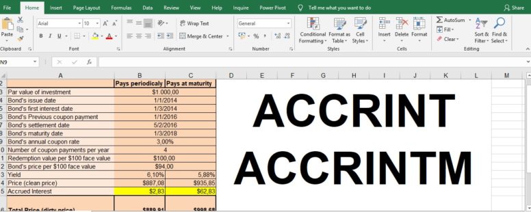
So in our example we see all the information of a bond we bought. The previous coupon payment was a few months earlier.
We have two scenarios for this bond. One that pays periodically and one that pays at maturity.
We have calculated the price in both of them using the Price functions. Take note here that the price functions return the per 100$ value so we multiplied this result by 100 to have the per 10000$ value which is the par value of our investment.
The par value is the face value of the investment, which is also called the principal of the investment.
In cell B14 and C14 we have calculated the clean price which is the price without the accrued interest. Below them we calculated the accrued interest and then the dirty price which is the total price of the bond, including accrued interest.
We have used both of the accrued interest function to achieve this. One for the bond that pays periodically, and the other for the one that pays at maturity.
To see how exactly we did this, let’s go to the next sheet where we have another bond for sale.
As we can see the accrued interest is yet to be calculated, thus the dirty price is still equal to the clean price.
We go to cell B15 to find out what the accrued interest for the bond that pays periodically is.
We type the name of the function, followed by the issue date and the first interest date. This is where we have to mold the function to our demands.
The ACCRINT function of excel, calculates the amount of interest that has been earned since the day that the bond was issued. This would not be correct, or fair to the buyer, since we would calculate in the accrued interest, money we had already received, up to the date of the settlement.
In our example we want to sell the bond in February of 2016 which means that we have already received all the coupon payments previous to that date. So the accrued interest should be calculated from the date of the previous coupon payment, which is the last we have received in January of 2016 up to the date of the settlement.
To mislead excel into doing our bidding we set as both issue date and first interest date of the bond the date of the previous coupon payment. This way Excel will think that the bond was issued on the date of the previous coupon payment and it will correctly calculate the accrued interest from that date to the date of the settlement.
So we select for the first two arguments cell B6. Then the date of settlement which is the date our sale is going to take place, the rate in cell B9, the par value of the investment in cell B3 and the frequency of payments from cell B10.
The next argument, basis, is optional and it helps us choose the type of day count to use. We will always use the default 0 value. And then the last argument, which is optional as well, is a logical value that specifies the way to calculate the total accrued interest when the date of settlement is later than the date of first interest. A value of TRUE returns the total accrued interest from issue to settlement. A value of FALSE returns the accrued interest from first interest to settlement. If you do not enter the argument, it defaults to TRUE. In our case both methods provide us with the same result since our issue date and first interest date are the same.
So we can omit both of the two last arguments. By pressing Enter we can see the accrued interest and notice that the total price has changed accordingly. Then we have to calculate in cell C15 the accrued interest for a bond that pays at maturity. We use the appropriate function ACCRINTM followed by its arguments. Here we don’t need to trick excel so we use the proper issue date from cell B4, and then the settlement date, the rate and the par value. We again omit the basis argument and we have our result and the total sell price of the bond in both scenarios.