Probably the easiest to understand lookup function is the CHOOSE function. It returns a value from an array of values, that corresponds to a specific position in that array.
Practice File:
Transcript
CHOOSE can have up to 254 value arguments.
Suppose we want to know the name of student with number 2 and we decide to use choose in cell B9.
We type the function name following the equals sign. Then we type the index number, which in our case is number 2 and then we type the values which in our case are the names for all three students. Cells B3, B4 and b5.
CHOOSE will return the second value from the supplied array which is Mary.
I know what are you going to say. Not impressive at all.
You are right. CHOOSE shines by helping other functions. By itself is not that impressive but with a little imagination and the help of some more functions, it can be a powerful ally to your battle with numbers.
The main reason for this is that its value arguments can be cell ranges and its return value can be a cell reference or a cell range reference as well.
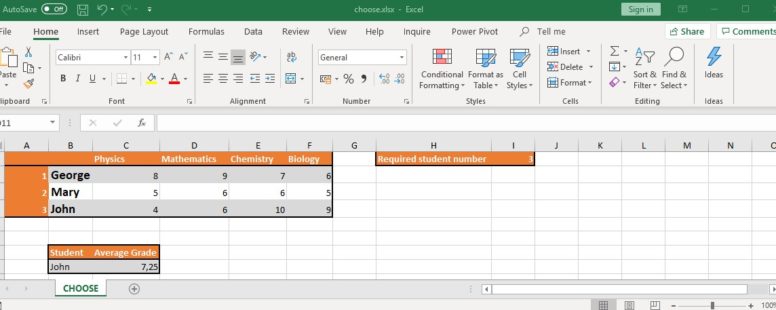
Suppose we need the average grade of a student to be calculated simply by providing their identification number.
CHOOSE can help us do that. Let us see how in cell C9. The number of the student we want to calculate the average for is found in cell I2. We have pre entered the value in I2. In real work circumstances this value could be calculated by other parts of our workbook or selected from a dropdown control.
Since we need the average we type the name of the function and then the cell range of values we want to calculate the average from.
We need the average of student 3 (john) so we could just select the cell range c5:f5, but every time the value in cell I2 changes we would have to manually recalculate the whole thing.
So instead we will use CHOOSE . We type the name of the function and the index number which in our case is the value of cell I2. Then we type the reference to the cell area of the grades of the first student (C3:F3), the second student and the third. We close the parenthesis and we have our result.
Now by simply changing the value in I2 we have a different average. We can improve our sheet more by making sure the name of the selected student is shown in cell B9.
In the function we previously typed in cell B9 we change the index number from 2 to cell I2.
Now every time the value in I2 changes the cells B9 and B9 show the name and the average score of the related student.
Of course there are plenty of ways to do the exact same thing in Excel, that are probably more productive but this was just an example for you to see how combination can completely change the role of a function and its usability.
One of the most interesting uses of CHOOSE is the ability to add extra functionality to the VLOOKUP function. We will show this on the lesson about the best lookup function to use.
There are plenty interesting uses of CHOOSE that one can find, with a little search, and even more, with a lot of imagination.