We will begin a quest to find the best lookup function. All the internal functions of Excel have limitations which we will try to overcome. In this and the following tutorials, the knowledge of the simple syntax of the functions mentioned (VLOOKUP, HLOOKUP, MATCH), is considered a requirement.
Practice File:
Transcript
The basic limitation of VLOOKUP and HLOOKUP is that they are single dimensional. They only search vertically or horizontally. The most obvious way to overcome this is by combining the two of them in a single formula.
In short we will try to make vlookup search in a matrix (both vertically and horizontally). To do this we will use a vlookup function with a nested hlookup to provide us with the column number attribute of the vlookup.
We will need to add a row of column numbers just below the headers of our columns as we can see on the current sheet.
In cell J we will look for the number of units sold on January 20 2015.
We have added row 2 which gives the number of each column.
We type our function using the value in J2 as the lookup value and the cell area A3:H44 as our lookup array. For the number of column, we will use the hlookup function.
We type the function and as lookup value we set the cell J1, and as lookup array the area A1:H2. We need the second row of data and of course the exact match. We need the exact match for the vlookup function as well. We press enter and there we have it a matrix lookup function using vlookup and lookup.
Although this combination works it needs us to create a new row with the column numbers. We can easily avoid that by using the match function instead of hlookup to look for the column number.
So we reached our next combination of functions Vlookup and Match.
On our next sheet we see the same data minus the extra row. We are going to try to achieve the same thing as before. In cell J3 we type the vlookup function with the same attributes as before but instead of hlookup for column we use the match function. We use the value in J1 as lookup value and the range A1:H1 as lookup array. We are still searching for the exact match so we type 0 for both functions and when we press enter we have the same result as before. A lot more elegant don’t you think?
One other limitation of vlookup is that it can only search for values to the right of the first column of its lookup array.
So if we wanted to search for the date that the units sold were 500 it would be impossible.
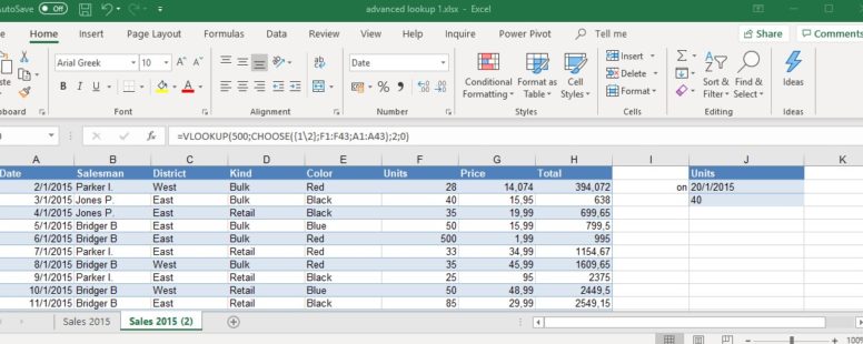
Choose gives us a kind of complicated way to achieve just that. We will stay on the current sheet and in cell J20.
We type the vlookup function, with lookup value of 500 and to define the lookup array we will use choose.
This syntax of choose uses as first attribute an array. This means that we want choose to select from the array variables all those with index in the given array in the first attribute.
Let’s type the function and try to explain it in plain language. We have given an array of two numbers as the first attribute. This means that we want to choose both variable number 1 and number 2 from the variables given.
The array variables given are the two columns. The one of units and the one of dates. Take note that as first column we have set the column of units and second the column of dates. So as far as vlookup is concerned it still searches to the right since the two column array we provided it with has the column units on the left and the column date on the right. We will need the second column in our vlookup function of course and the exact match. The result is what we would expect and vlookup has a new functionality.
We might be able to accomplish this for a matrix lookup as well but I wouldn’t even try it. There are a lot better ways to achieve this and we will talk about them in our next lessons.