When you start learning about the lookup functionality of Excel, VLOOKUP will probably be one of the first functions you will stumble upon.
Practice File:
Transcript
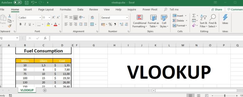
We will continue with the VLOOKUP function. In cell area B4 to D12 we can see the fuel consumption and the cost in dollars, for certain distances calculated in miles.
For example, for a 75-mile journey we need 10 liters of gasoline which cost 13 dollars.
Let’s suppose we want to look up the consumption in liters for a 100-mile journey and show it in cell H14. In such a small pool of data it is relatively easy to find the proper value and manually type it in the proper cell.
Imagine if your data spanned to thousands of rows and columns. Finding out the needed value then, could be impossible.
This is where Excel’s lookup functions provide us with the solution.
So in cell H14 we will use the vlookup function to get the value we need.
The vlookup function searches the data of the first column on the left of the cell area B4:D12 for a value, in our case it is 100, and returns the value of the cell that can be found at the same row, and at a given column of the cell area. In our case the column is the second one and so the value is 15.
We select the cell and navigate to the Formulas tab. We click at insert function and set the category to Lookup & Reference. We locate the VLOOKUP function and click OK. We can of course just type the name of the function after the equals sign.
At the arguments window, we set the value that we are looking for at the “Lookup_value”. We select the cell F14, which refers to the distance that we are looking for, the 100 miles.
At the field “table_array” we need to define the cell area where Excel will perform the search; this is the cell area B4 to D12. At the argument “Col_index_num” we define the column number where the liters are displayed. In our case this is the second column, so we type the value 2.
The last field contains only two options: TRUE & FALSE. We can type the number 1 or 0. If we type the number 0, Excel will only look for an exact match. In case there is no such value, Excel will display an error message. If we type number 1 and there is not an exact match, Excel will find the lower closest match in the first column. In our case it would be 75.
We need to note that in order to use this function with the last attribute set to 1, the cell area needs to be sorted in ascending order by the column in which we want to look for the value. In our case by the column “miles”.
We type 0 and click at OK. As a result, the value 15 will be shown, which corresponds to 100 miles.
If we change the value of the cell F14 to 110 miles, we can see that an error message appears because there aren’t any values available for 110 miles.
The letter V at Vlookup stands for Vertical. So, VLOOKUP looks for a value, in our case 100, at the first column of a cell area, and when it finds it, it returns the value that is found at a cell with the same vertical position and on the right of the first column.
In our example, we have asked for the second column, that’s why we had the result 15. In case we had asked for the third column, we would have the result 19.5.