One very useful Excel function is OFFSET. It returns a range of cells which corresponds to a specified number of rows and columns starting at a given distance from a reference cell.
Practice File:
Transcript
Sounds complicated, but only until we see it in action.
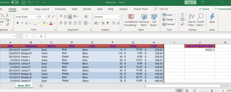
Suppose we want to calculate each day the sum of the 10 largest sales. (the ones which produced the greatest income).
Sounds easy we just sum the 10 last values of the total column of our table since it is sorted in ascending order by that same column.
Well that is correct, but it also means that each day when new sales will be added we would have to do the same thing again.
Offset can give us the solution since it can give us the last 10 rows of the total column, if we just provide it with the total number of rows of data.
Since the data change every day to know what the last row is requires the use of one more function. The countA function counts the numbers on a specified range. So if we use it for column H it will return us the count of numbers in that column, thus the total number of rows of data.
We keep this number on this cell and we will use a reference to it on our offset formula for simplicity.
Now it is time for the magic.
In cell J2 we will use the offset formula to calculate the sum of the 10 largest sales.
First we type the sum formula and nested inside it the offset formula.
We type the name of the function and then we have to type a reference cell. This could be any cell in our sheet but usually we select the first cell of our table, which is a1.
Then we type the offset of the first row of our required data range. This is calculated by the value we found before, in cell K11, minus 10 since we want the last 10 rows of data. Then we type the offset column. Since we are currently on column 1 (the A1 cell) and the data range we need is on column 8 (the total column) the offset is 7 (1+7=column 8).
So we have successfully directed our offset function to the beginning of our data range which is cell H34. Now we only have to set the height to 10 (the 10 largest sales) and the width to 1 since we only need the total column.
We press enter and we have the desired result.
This cell now calculates dynamically the 10 largest sales of our company.
Excel provides us with a lot more ways to do exactly the same thing, either with tables or with the index function, but offset has its uses. Even if we decide to use another function for the given example, no one can deny the usefulness of offset which in combination with other functions can provide elegant solutions to complex problems. We will see on later lessons a very efficient way to lookup values with the help of offset.