Excel has provided us with several functions, to help us make sense of huge pools of data. AVERAGEIFS is one of them.
Practice File:
Transcript
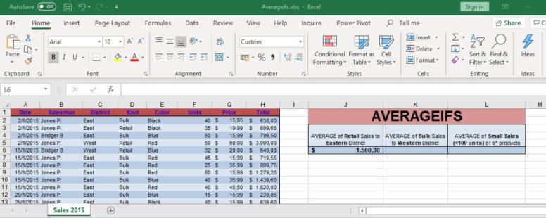
In the current worksheet we can see a small example of the data we need to handle.
This is the sales of a company for the year 2015.
We have the date of the Sale, the salesman, the district at which the sale took place, the kind of sale (bulk or retail), the type of the product (in this example we only differentiate the products by color), the units sold, the price per unit, and the gross total of the sale.
Of course at a normal working environment these data would only be a tiny fragment of the actual data we would have to analyze.
We have already calculated, using AVERAGEIFS, the average of the gross total of the retail sales to the eastern district in cell J6.
Without AVERAGEIFS such an automatic calculation would be impossible and the manual one would require several workhours.
Let’s suppose now that we need to calculate the average of the gross total of the bulk sales to the western district in cell K6 using AVERAGEIFS.
We select the cell and type the equals character followed by the name of the AVERAGEIFS function and a left parenthesis.
Then we enter the cell area we need to calculate, in our case the area from H2 to H43.
After that we define the cell range of our first criterion, in our example this is the column of the kind of sale, from D2 to D43.
Following is the criterion for this cell range. The criterion is that the type of sale is bulk, so we type, inside double quotes, equals Bulk. We should note here that we can omit the equals sign if we want.
Then we proceed to our next criterion.
First we pick the cell range, from C2 to C43 and then the criterion which is the Western district. Take note that we chose not to use the equals sign now.
Our function is ready and if we close the parenthesis and press enter, we will see the result which is 1200 dollars.
Following the same syntax, we can use up to 127 criteria ranges and criteria in a AVERAGEIFS function.
Let’s see one more example in cell L6, where we have to calculate the average of the gross total of the small sales of products with color name starting with the letter b.
We type our function, the average range same as before and our first criterion range, in this example the cell area from F2 to F43.
Then we type the criterion less than 100. We cannot omit the less than sign of course since this is only valid for the equals sign.
And then as before we proceed to our second criterion.
Let’ s note here that we have to use wildcards to our criterion. We use b followed by an asterisk sign, thus including both color blue and black in our calculation. Then we press enter, which shows our desired result.