Use LOOKUP when you need to find something in a single row or column and find a value from the same position in a second row or column.
We have prepared a tutorial on the LOOKUP function to explain it in a bit more detail.
There are two ways to use LOOKUP function. The vector and array form. The array form of the function is provided only for compatibility with other spreadsheet software and is not recommended from Microsoft. So we will only focus on the vector form here. You can achieve the functionality of the array form of the LOOKUP function a lot more efficiently using the other 2 lookup functions VLOOKUP, HLOOKUP.
The syntax of the function is the following:
LOOKUP(lookup_value, lookup_vector, [result_vector] )
lookup_value : The value that you want to match in lookup_vector.
lookup_vector : The range of cells being searched. It contains only one row or one column.
result_vector: Optional. A range that contains only one row or one column. It has to be the same size as the lookup_vector.
If it can’t find the lookup_value, it matches the largest value in lookup_vector that is less than or equal to lookup_value.
If lookup_value is smaller than the smallest value in lookup_vector an error #N/A is returned.
Click on the button to practice using this function, with the help of our Online Assessment Tool:
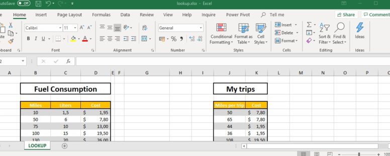
Here is an example of how to use the LOOKUP function:
Use the Lookup function to display in the cell C20 the value of the Column C that corresponds to the letter of the Column A, according to the letter displayed in the A20 cell. The table range is A1:C18.