From all the lookup functions, LOOKUP is the least useful. Even though it is a powerful function, it is hardly used at all.
Practice File:
Transcript
We will continue with the lookup function. The lookup function has two forms. The Vector form and the array form.
Microsoft proposes not to use the array form and use their two other lookup functions. VLOOKUP and HLOOKUP.
But in truth, although it is a powerful function, lookup is hardly used at all.
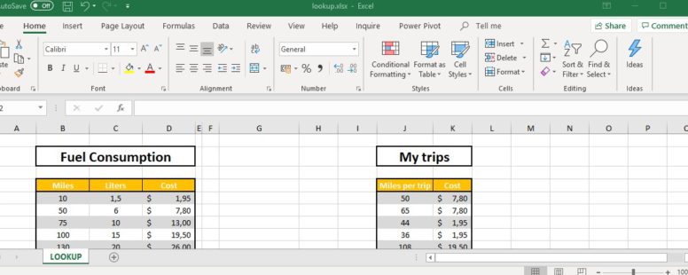
In cell area B4 to D12 we can see the fuel consumption and the cost in dollars, for certain distances calculated in miles.
For example, for a 75-mile journey we need 10 liters of fuel which cost 13 dollars.
Let’s suppose we want to look up the consumption in liters for a 100-mile journey and show it in cell H14. In such a small pool of data it is relatively easy to find the proper value and manually type it in the proper cell.
Imagine if your data spanned to thousands of rows and columns. Finding out the needed value then, could be impossible.
This is where Excel’s lookup functions provide us with a solution.
In order for the lookup function to work properly in either of its forms the column with the data we will be searching must be sorted in ascending order. Also the value we need to search for cannot be lower than the lower value of this column, or an error will occur.
The lookup function searches the data of the first column on the left of the cell area B4:B12 for a value, in our case it is 100, and returns the value of the cell that can be found at the same row, and at a given column. In our case the column is column C and so the value is 15.
So in cell H14 we will use the vector form of the function to get the value we need.
We select the cell and navigate to the Formulas tab. We click at insert function and set the category to Lookup & Reference. We locate the LOOKUP function and click OK. We can of course just type the name of the function after the equals sign.
At the arguments window, we set the value that we are looking for at the “Lookup_value”. We select the cell F14, which refers to the distance that we are looking for, the 100 miles.
At the field “search_table” we need to define the cell area where Excel will perform the search; this is the cell area B4 to B12. At the argument “results_table” we define the column number where the liters are displayed. In our case this is column C.
If we use the value of the cell F15 in cell H15, we can see that the result remains the same, because if an exact match is not found, the Lookup function will match the closest value below the lookup value.
The array form of the function is a bit more complicated. It takes two attributes. The first is the lookup value and the second is a table of data containing values to be searched in the first row or column and values to be returned in its last row or column.
Suppose we want to approximately calculate the cost of fuel for our monthly trips in cell K5 to K12.
First we select the cell range K5:K12 and then we type the equals sign followed by the name of our function. The fist attribute is the lookup values which in our case is the cell range B5:b12.
We said that this form of lookup chooses its results from the last column of the given array. So since we want to show the cost for the given mileages, the last column of the given array should be column D. So we select B5:D12.
We will use this as an array formula so we have to remember to press ctrl shift and enter instead of just enter.
We can see that the approximate cost for each trip is shown in its proper place.
If instead of cost, we needed to show the liter consumption then as the second attribute of the lookup function we would provide the cells B5:C12.