In another tutorial we saw how we can find ourselves a better loan for a new car, using Goal Seek . Although Excel’s Goal Seek is a powerful tool, it has one basic limitation. It allows only one variable to be changed to help us achieve our goal.
Excel provides an even more powerful tool that bypasses this limitation. The Solver. The Solver is in the form of an add-in which must be enabled before you can use it.
Practice File:
Transcript
Let’s see how to do that first.
We click on the file tab of the ribbon, and then on options. Then select add-ins, and from the dropdown list on the bottom right we select Excel Add-ins. We click on Go and a popup window appears which contains a list of add-ins. We tick the box with the solver add-in and press OK. At the end of the data tab of the ribbon a new button has just be added by the name solver.
Let’s test it.
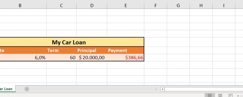
In our example we are planning on buying a new car and have our eyes on a certain model with a cost of 20000$.
Unfortunately, we don’t have the money and have to turn to a bank for a loan.
The initial offer from a banker is shown in the current spreadsheet.
The rate is 6% per year for 5 year monthly payments (60 payments in total).
As we can see the monthly payment needed to fill the requirement is about 386$.
This happens to be over our budget and we want to explore more possibilities.
We feel that we cannot pay more than 300$ per month, but we can handle a bigger duration of the loan, but up to 80 months.
Also the interest should not exceed 6%.
In such a small scale example we could have used goal seek multiple times until we reached the desired results. With solver we are a lot more flexible. We click on our newly added button.
In Set Objective field we set cell E7.
In the “By changing variable cells” field we provide the cells that can be changed to achieve our objective. These are cells B7 and C7.
Now we can add our required restrictions.
First the required monthly payment to -300 in cell E6.
Then the annual rate to less than or equal to 6%.
And finally the number of months to less than or equal to 80.
Before we click on solve let’s have a small tour of the interface. Below the add button are the buttons to change or delete one of the added constraints. Then it is the button to reset all constraints, followed by the button to load or save a set of constraints for future use.
By clicking on the options button we have access to various options of the solver add-in. Let’s review some of them.
The constraint precision, which defines the steps of the values of each constraint, in order to reach our objective. A smaller number increases the precision of our calculation but in larger scale projects can vastly increase the time of execution.
The “show iteration results” is the option to use if we need to access all the evaluation steps of the solver add-in.
Automatic scaling makes sure that extreme values are not used for the solution of the solver (for example one monthly installment of 20000 dollars with zero interest). So we select it and press ok.
Since our problem is non-linear we will choose the non-linear method and click on solve.
A new window appears. On the left we have the option to keep the solution or revert to the original values, with a checkbox just below to return us to the solver window. On the right there are a number of reports the solver add-in can produce and store on separate worksheets.
Since we are satisfied with the supplied solution we press ok.
The solver add-in has a vast array of applications. We cannot cover all these in this lessons but, hopefully you learned enough to be able to use and eventually master it.